Digital Audio

The music library operated at a high level of abstraction in the sense that it provided a “vocabulary” of manipulating sound—note, par, seq, etc.—directly in terms of what we were creating: musical compositions. Such a high level approach to programming is preferable whenever possible because it allows our programs to better directly reflect our intent. However, while a high level of abstraction better directly reflects intent, it lacks in flexibility. What if we didn’t want to create music? Instead, what if we were concerned with generating audio that was not necessary “musical” in nature? The music library simply does not provide us any way to manipulate sound beyond the “language” of music!

Instead of using music, we need a lower level view of what sound is, so that we can manipulate it in a variety of ways. In this reading, we’ll introduce how we represent audio in a computer program and how that representation maps onto a data structure we’ve already worked with extensively, the list.

What is Sound?

Before we talk about representing sound, we first need to understand what sound is precisely! In short, what we perceive as sound is vibrations in the air. These vibrations take the form of acoustic waves that propagate from a sound source, through the air, and to our ears. The following visualization from an NPR article on what sound looks like illustrates the acoustic waves generated by a speaker:

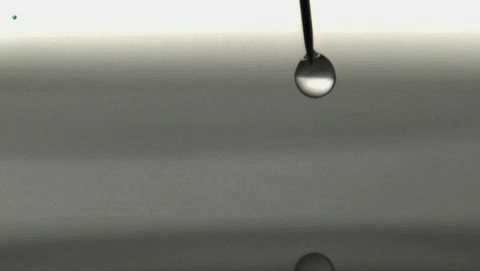
Note how similar the acoustic wave from the speaker looks to the waves generated from a water droplet:

The following video from the same NPR article also gives an excellent visualization of acoustic waves:

• https://www.youtube.com/watch?v=px3oVGXr4mo

We can describe the motion of such a wave as a two-dimensional plot where the \(x\)-axis represents time and the \(y\)-axis represents the pressure of the wave, the amount of force exerted by the sound source to the surrounding air.

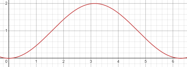
As we shall see, simple waves such as the sine wave above create “pure” sounds to our ears. The more complex sounds we hear in everyday life can be thought of as the combination, or superposition, of many different sound waves.

How Do We Represent Sound in a Computer?

The amount of pressure that a sound source creates over time is a continuous function, i.e., the pressure changes over time in a smooth fashion without any discontinuities. This is immediately a problem for us as a programmer: we can’t represent continuous functions precisely in a digital computer! Why is this? If there are no discontinuities in the function because it is continuous, that means that it is infinitely divisible, i.e., for any two data points generated by the function, there always exists a point “in-between” those two points. This immediately implies that to store the result of a continuous function, we would need an infinite amount of memory. But memory is a real, physical commodity in a computer, so we can’t have an infinite amount of it! (N.B., the “digital” in “digital computer” indicates this fact. All data in a computer is discrete, i.e., discontinuous, in nature!)

So what can we do? Well, rather than representing all of the values of this continuous wave, we will instead choose a finite number of samples from the wave. Each sample is a single integer describing the magnitude of the pressure at a given point in time. Below is an example of us choosing to sample the wave at every \(0.2\) units of time to approximately \(2\pi\).

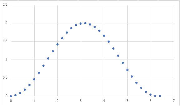
Note that this choice of the number of samples allows to approximate the shape of the continuous wave quite well. However, a different choice may not net as good of a result. For example, here’s what the wave looks like if we sample at every \(1.0\) unit of time.

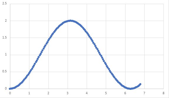
It isn’t clear that our data captures a sine wave at all! When we use even more samples, e.g., \(0.05\) units of time, it becomes very obvious we are approximating our original sine wave.

But perhaps that was overkill? We could definitely approximate the shape of the wave using less samples!

Because each sample is captured by a single integer, we must carefully choose the amount of samples we are willing to make when representing audio. More samples lead to more accurate sound, but take up more memory!

Assuming we know the sample rate, i.e., the interval at which we sample data from the sound wave, we can represent sound as a list of integers. Here are lists of integers corresponding to the three waves given above:

(define example-digital-wave
  (|> (range 0 (* 2 3.14) 0.2)
      (lambda (l) (map (lambda (x) (- x (/ 3.14 2))) l))))

(define example-digital-wave-less-samples
  (|> (range 0 (* 2 3.14) 1)
      (lambda (l) (map (lambda (x) (- x (/ 3.14 2))) l))))

(define example-digital-wave-more-samples
  (|> (range 0 (* 2 3.14) 0.05)
      (lambda (l) (map (lambda (x) (- x (/ 3.14 2))) l))))

(length example-digital-wave)

(list-take example-digital-wave 10)

(length example-digital-wave-less-samples)

example-digital-wave-less-samples

(length example-digital-wave-more-samples)

(list-take example-digital-wave-more-samples 10)

Characteristics of a Sound Wave

Now that we know how we’ll represent digital audio (as lists of integers), we can now talk about the characteristics of a sound wave that shape how we perceive the sound. Throughout our discussion, we’ll illustrate our waves as continuous functions, but remember our representation is merely an approximation of them!

The form of a wave is the shape of its repeated pattern. A sine wave, like the one above, is called so because its form follows the repetitive nature of the mathematical \(\sin\) function. In terms of acoustic properties, the shape of the form broadly determines the timbre or quality of the sound, e.g., is it harsh or soft sounding?

In addition to the waveform, there are two other important properties of a wave that governs how we “hear” it:

• The frequency of a wave is the number of times the waveform pattern repeats over a fixed time interval. We typically measure the frequency of a wave in hertz (Hz), repetitions per second. The frequency of a wave governs the pitch of the sound we perceive, e.g., is it a low tone or a high tone?

  Alternatively, we can talk about the period of the wave: the duration of a single pattern. Note that period and frequency have an inverse relationship: frequency (patterns per second) is the inverse of period (seconds per pattern)!

• The amplitude of a wave is the height of its largest peak. We measure the amplitude in decibels (dB), a “unitless” quantity describing the ratio between two values (on a logarithmic, base-10 scale). In terms of sound waves, this ratio is the “rest state” of the medium the wave propagates through and its peak. The amplitude of a wave governs how loud the sound is.

Thus, we can generate different kinds of sounds by varying:

• The waveform to get different sorts of tones.
• The frequency to obtain different pitches.
• The amplitude to vary the loudness of the sound.

In lab, we’ll look at creating different sounds using Scheme, a process called sound synthesis!

Self Checks

Problem: Exploring Sampling Rate (‡)

As discussed in the reading, choosing the sample rate of an audio clip is an exercise in trade-offs: audio precision versus storage space. To get a concrete feel for these trade-offs, watch this video illustrating the differences in encoding audio as we vary two values:

• The sample rate as we previously discussed in the reading is how often we record values from the sound wave.
• The bit depth is the size of the range of values we capture per sample.

If a lower sample rate causes discontinuities in the axis of time, a lower bit depth causes discontinuities in the axis of pressure. With a smaller range of possible values, we cannot capture nuances between differences in pressure between samples.

• All The Sample Rates: https://www.youtube.com/watch?v=6kIHsGJSUrY

Watch the video and in your reading response, simply note the highest bit depth and sample rate where you perceive no difference in the sound relative to highest values (16 bits, 44.1 kHz sample rate). For fun, if you have a digital music collection, you might want to revisit it and see what the bit depth and sample rates of your music files are! Do you have any files that have low bit depths or sample rates? Can you tell the difference?